Our new Address: http://www.bsc.es/viz/corner/
Inequality and economic growth in Argentina
A small clarification before we start: I am not pro or against the current Argentinian government, and if I had to vote in next sunday’s elections I would not be able to choose a side. The following is not a real political commentary, what I like is data visualization.
Recently I got to read Alberto Cairo’s The Functional Art, and I was strongly attracted to a great infographic about the evolution of the economy and inequality in Brazil. It got me thinking about how would that look for Argentina, so I went and got the data from the World Bank (starting in 1986, and only up to 2013), and reproduced the plot in a very similar style but using the Argentinian data.
Link to the original plot and discussion
My plot:

The chart’s interpretation is that points higher up represent more inequality, while points to the right mean a higher production of economic value. In the words of Alberto Cairo, one of the messages of the chart is that growth in GDP does not always mean a reduction in inequality.
A few technical comments:
Like in the original chart, I used the Gini coefficient to measure inequality. It is far from a perfect indicator, but it is a very popular one. To measure economic growth I decided to use the GDP per capita instead of the total one used in the original chart. I think this would be a little better since the country’s population grew significantly in the three decades spanned by the data.
I respected the original design and separated the presidential terms by colour, which I think is a brilliant decision. It totally makes the plot. There is one caveat though, and it is that each data point measures a whole year and president changes happen at different points during that year. Therefore there might be some leeway in how to put the color (and I did’t figure out an impartial algorithmic way to decide this).
With the risk of ruining the incredible work by Cairo and collaborators, I took the liberty of adding a few labels indicating important economic events (and I also changed fonts, colors, stroke widths, and other small stuff that makes my chart subtly but clearly worse, of course).
Comments on the content:
Like in the original chart, you can see a clear mark or general tendency that is very different for each presidency (including the difference between Menem’s first and second term).
More importantly, beginning in 2003, and coinciding with the Kirchner’s rise to power –just like Lula in Brazil–, the country grows economically and inequality goes down in an unprecedented manner (except for a small glitch under the global economic crisis of 2008). I could not find Gini estimates before 1986, but there are some for the urban area of Buenos Aires and they show that only in 1984, and before that in 1974, there were such low levels of inequality as today.
An important detail: reliability of the source
After a lot of comments by many of the readers in the original (in spanish) post, I caved and gave more hours to this project and included an alternative measure of GDP (alternative to the World Bank, that is).
Why? Well, for those not well versed in Argentinian politics, the current government intervened the official statistics institute, and since then their numbers (which feed the World Bank’s database) have been strongly questioned by many. The World Bank itself recognises that unreliability of the official data from Argentina and puts a disclaimer saying «the World Bank is also using alternative data sources and estimates for the surveillance of macroeconomic developments in Argentina».
Many people asked me to get an independent source and check the data, so I did. I discovered other things in the middle, like for instance that it is terribly difficult to match different methodologies when measuring GDP. Therefore, I decided that the best (in terms of a compromise between easiness and correctness) was to give the official numbers for 2007 as valid, and then calculate the subsequent years from the relative growth (year to year percentage) measured with this other indicator (called ARKLEMS, it just rolls of of the tongue right?). The data from this analysis is shown in the alternative timeline in gray, which unexpectedly (from the comments), almost lines up with the data from the World Bank.
There are still things that bother me with this: first, I am plotting different things that maybe have no way of being normalized to the same values, and second, and perhaps more important, perhaps this indicates that the adjustment was already taken into account by the World Bank in my original data set (they say they are doing it, but not how). Hopefully this will lead to good conversations and discussions on how to recover the reliability of the INDEC.
New questions:
The evolution in Brazil, the original chart, is strikingly similar to that of Argentina. This makes me wonder how much is the effect of particular presidents (sure there must be some, but still) compared to the global and regional environment. To answer this question I got the full data set from the World Bank and maybe in one or two weeks I’ll get a complete infographic with a comparison (it won’t be easy as I have to rethink the design and maybe even go interactive…)
Note:
All the data comes from the World Bank, from this table and this table, except for the Gini coefficient from 88, 89, and 90, which I found in Gapminder.org. They cite the World Bank as a source but probably they took it from somewhere else. As a side note, Gapminder already let’s you do the comparison between countries of the region, only that there is no presidencial term information. The alternative GDP calculation from 2008 onwards was taken from ARKLEMS, which I adjusted for population growth, and only used the year to year change to estimate the movement of the 2007 World Bank data point.
Desigualdad y crecimiento económico en Argentina
Antes que nada: No soy pro-Kirchner ni pro-Macri, y honestamente si hoy tuviera que votar en Argentina no se a quién votaría. Esto no es un comentario político real, a mi lo que me gusta es la visualización de datos.
Hace poco leí en profundidad el libro de Alberto Cairo El Arte Funcional, y me atrajo una infográfica muy buena acerca de la evolución de la economía y la desigualdad en Brasil, y me dió curiosidad saber como serían esa gráfica para Argentina. Después de conseguir los números del Banco Mundial (solo conseguí datos a partir de 1986, y solo hasta 2013), reproduje la gráfica en un estilo muy similar pero utilizando los datos para Argentina.
El mío:
La interpretación de la gráfica es que puntos mas arriba representan una distribución mas desigual de los ingresos, mientras que mas a la derecha significa una producción total de riqueza mayor. En palabras de Alberto Cairo, vemos que «un crecimiento del PBI no siempre está acompañado de una reducción de la desigualdad».
Un par de comentarios técnicos:
Como la gráfica original, para medir la desigualdad uso el coeficiente de Gini. No es una medida perfecta pero es un indicador muy utilizado. Para medir el crecimiento económico decidí usar el producto bruto interno per capita, introduciendo un cambio con respecto a la gráfica original (que usa el producto bruto interno total). Me parece que es un poco mas correcto usar esta gráfica ya que el tamaño de la población cambió bastante en las tres décadas abarcadas por los datos.
Respeté el diseño original de separar los datos en intervalos por presidencias, una decisión de diseño brillante. Sin embargo, creo que como la medición de cada año es para el pasado, y los cambios de presidencia están marcados aproximadamente dentro de ese año, se introduce un poco de ruido y el punto medido no coincide en realidad con la separación de colores perfectamente (a ver si se me ocurre un criterio automático para solucionar esto).
A riesgo de arruinar el increíble trabajo de diseño de Alberto Cairo y sus colaboradores, me tomé la libertad de agregar pequeños recordatorios de eventos económicos importantes de cada año (además de cambiar fonts, colores, anchos de líneas, y otras cosas que hacen que mi gráfica sea claramente peor, por supuesto :).
Comentarios sobre el contenido:
Como en la gráfica original, se puede ver una clara marca o tendencia general muy diferenciada por cada presidente Argentino (incluyendo Menem primera o segunda presidencia).
Mas importante, a partir de 2003, coincidiendo con la entrada de los Kirchner en el poder –y así como en Brasil con la entrada de Lula–, el país crece económicamente y baja la desigualdad de manera sistemática y sin precedentes (excepto por un retroceso coincidiendo con la crisis financiera global). No existen mediciones del índice de Gini a escala del país antes del 86 (o no las encuentro), pero las calculadas para Buenos Aires dan que no se veían niveles de desigualdad tan bajos desde 1984, y eso es un punto bajo especial que solo tenía pareja en 1974 (datos de Gapminder).
Nuevas preguntas que surgen:
La evolución en Brasil es muy similar a la de Argentina. Esto hace que me pregunte cuanto es el efecto de los presidentes en particular (que seguro hay alguno) y del comportamiento económico global y de la región. Para responder esta pregunta me bajé los datos de los países vecinos de Argentina, y voy a crear (tal vez dentro de una o dos semanas) una infográfica mas completa comparando todos los países (que me va a llevar mas esfuerzo porque no es fácil poner en la misma gráfica a Brasil y a Bolivia, por ejemplo). Próximamente por este blog…
Edición posterior:
Repito para responder antes que sigan preguntando: Todos los datos salen del Banco Mundial, de esta tabla esta tabla y de esta otra, excepto por los años 88, 89, y 90 del Gini que están sacados de la estimación de Gapminder.org, que cita al Banco Mundial como su fuente pero probablemente lo sacaron de otro lado. De paso comento que con Gapminder ya se puede hacer la comparación de países de la región, pero no hay información de los períodos presidenciales.
Segunda Edición: actualización con nuevos datos del PBI alternativo
ESTA SECCIÓN HA QUEDADO ALGO INCOHERENTE, VER EDICIÓN POSTERIOR MAS ABAJO
Por un lado me encanta la increíble recepción que ha tenido este artículo, pero por el otro me han llenado ya demasiado la cabeza con el tema de la confiabilidad de los datos del INDEC (y por ende, de los de mi fuente que es el Banco Mundial). Esta desgracia institucional me ha hecho sacar horas de donde no las tengo buscando como incorporar en la gráfica algo de este tema. Aqui está, pero antes, unas (cuantas) palabras.
No estoy contento del todo con el resultado por dos motivos, y ninguno tiene que ver con lo que dicen los datos: (1) Me molesta que la nueva presentación gira la discusión hacia el problema del INDEC y la mentira institucional. La gráfica original de Cairo tiene como tema principal la correlación entre el crecimiento económico y la distribución de la riqueza. Invita a pensar en la personalidad que cada presidencia dió a estas variables, a la comparación entre épocas y a ponerse ansioso y querer saber que le pasa a otros países. Técnicamente hablando, lo que ocurre ahora es que al mostrar dos conjuntos de datos para una misma secuencia, nuestro cerebro automáticamente entra en modo comparación/busqueda de similitud y diferencia, y el tema original se reemplaza por este. Para mitigar este problema resolví usar otro código de color (gris) para esta línea alternativa, intentando mantener la primera historia en una primera capa, y la segunda que aparece cuando hemos ya pasado por la primera. Es un intento de narrativa por capas, o como se llame, pero no se si me salió bien.
(2) Como visualizador de datos, lo mejor del mundo es tener una fuente confiable, regular, o por lo menos completa, de manera que puedo focalizar en construir el mensaje visual, en como se va a leer, en crear estructura gráfica y luego diseñarla, que son las cosas que me apasionan. Cuando los datos vienen «sucios», como decimos, hay que hacer un buen trabajo de normalización, inspección, etc, lo que llamamos «limpieza», repasando 17 veces para que no se escape ningún maltrato del dato o error estadístico. En este caso estoy combinando dos fuentes de datos que incluso puede que no sean completamente compatibles, y el resultado es que estoy poniendo juntos en la misma gráfica cosas que no estoy seguro si deberían estarlo (porque no soy un experto). Al final, que si esto fuera un periódico o una publicación con una editorial fuerte, nunca publicaría esta nueva versión, porque técnicamente agrega mas problemas de los que soluciona. Pero como esto es un blog sobre visualización experimental, y aquí la audiencia ha demostrado un altísimo nivel de poder ver las historias y los detalles de la primera versión, voy a dejar la original que me gusta porque tiene menos cosas, y poner aquí la nueva para que sigan discutiendo (la metodología la explico mas abajo):
(aqui estaba la imagen con los datos de ARKLEMS, ver mas abajo)
Con respecto a la fiabilidad de los datos anteriores y de los nuevos. Como comentó uno de los lectores, el mismo Banco Mundial (que usa datos del INDEC) reconoció que era una fuente de datos no confiable a partir del 2007, en especial para los datos de PBI. Sin embargo, a partir del 2014 volvieron a incluír las estadísticas, mencionando que el FMI todavía tiene a Argentina retada por no producir buenos datos, y que en ese contexto «el Banco Mundial también usa fuentes de datos y estimados alternativos para la supervisión de los desarrollos macroeconómicos en Argentina» (traducción mía de la errata de Abril de 2014). No me queda claro de este mensaje si el Banco Mundial solo mira esos datos alternativos, o si los incorpora en sus publicaciones y por lo tanto los datos originales que utilicé ya están corregidos.
Supongamos que no. Me sugirieron usar el indicador de ARKLEMS, creado y mantenido por un grupo de profesores de la UBA. La verdad es que no conozco cuales pueden ser mejores o peores, o si hay mas, asi que vamos a ir con este que tiene un nombre llamativo y fácil de recordar :). Cómo pegarlos? Son fuentes muy dispares en su metodolgía y la salida final, asi que hay procesarlo un poco (lo que mencionaba arriba). Después de darle varias vueltas para ver como juntarlo, decidí que lo mejor (en términos de balancear facilidad de implementación y comprensión con correctitud) fue utilizar el último punto que se considera válido del Banco Mundial (2007) como el punto de empate entre las curvas, y calcular la evolución de ese punto en adelante usando los crecimientos porcentuales año a año reportados en ARKLEMS. O sea, la curva gris que está en el nuevo gráfico se va calculando año a año a partir del año anterior y del cambio registrado en ARKLEMS. Es decir a partir de 2007 no se utilizan más los datos del INDEC.
¿Que cambia? Bueno, como era de esperar, hay menos crecimiento. La crisis del 2008 pegó mas fuerte de lo se veía antes, el crecimiento entre 2009 y 2011 fue grande pero no tanto, y a partir de 2011 se estanca el crecimiento. De cualquier manera la curva sigue mostrando un crecimiento, mas moderado, y más importante, la caída de la desigualdad, ya que este indicador es independiente y nunca dejó de ser aceptado por el Banco Mundial. Un poco sin sorpresas, la tendencia general permanece similar, por lo que la historia contada en la primer versión era básicamente correcta. Es mas, uno de los comentarios estimaba que el PBI final iba a caer cerca de los 9000, muy buen ojo!
Bueno, esa es mi interpretación. Opinen lo que quieran, pero como siempre manteniendo el respeto por favor, que venimos bastante bien.
Por útlimo, vuelvo a repetir que lo que me gusta es la visuaización de datos, y aunque no esté conforme es cierto que esta nueva gráfica me trajo un par de desafíos interesantes en ese sentido. Espero que si un poco falla y nos hace dejar de hablar de que pasó con la economía Argentina, al menos nos lleve a buenas discusiones sobre como recuperar la confiabilidad del INDEC, que sería muy bueno.
Aprovecho para agradecer todos los comentarios, pero por favor por unos días no pidan mas cambios 🙂
Un saludo
TERCERA EDICION: O sobre como cagarla, y luego reconocerlo.
El gráfico que presenté originalmente tenía un error mío, interpreté «USD a valores actuales» como USD ajustados por inflación a valores de hoy. Ahora la gráfica es correcta (la que está arriba), con valores USD constantes a 2005. La anterior está mas abajo luego de la discusión de mi error.
A ver, tengo que pedir mil perdones por cometer un error básico. Esta vez los dioses de la estadística me sonrieron y la gráfica no cambia sustancialmente (también porque la tendencia es mas fuerte que la correción), pero es importante reconocer que la cagué y arreglarla. Por si no se nota, me siento mal al respecto.
Mi error, que astutamente reconocieron algunos lectores en sus comentarios, fué interpretar la descripción de los datos «USD a valores actuales» como USD ajustados por inflación a valores actuales. Los valores ajustados siempre se dan en referencia a algún año en concreto, pensé que buenos estos tipos me los dan a valores 2015. Pues no.
La nueva tabla de PBI que estoy usando es esta.
La gráfica correcta está arriba de todo, aquí abajo la primera que hice (solo le he cambiado la leyenda para que no circule mas la original con el error), para comparación.

Dos cosas: 1) Es notable que a pesar de cambiar los números, el comportamiento general de cada una de las presidencias que se veía en la otra curva se mantiene, y 2) Estoy asombrado con como coinciden los porcentajes de crecimiento año a año de la medición independiente de ARKLEMS con los datos del Banco Mundial. ¿Será que están realmente ajustando los datos del INDEC con indicadores alternativos? Para recordar, en esta curva tomo el valor 2007 del Banco Mundial como bueno, y le aplico el crecimiento año a año medido con el ARKLEMS per capita (porque ARKLEMS está en pesos y no quiero ponerme a usar tasas de cambio varias). La otra opción es que el INDEC está publicando bien los números y solo lo ha quedado la mala fama, que sería un primer paso para recuperarla. O por supuesto puede que la metodología de ajuste de ARKLEMS a esta escala no sirva, por ahora no me doy cuenta de como. Si alguien quiere ayudar en eso, bienvenido.
The UX Visualization Diaries · Number 1
Someone once accused me of not doing visualizations. Although that is not actually true (I’ve done more than one and so that means there are a lot of people out there with a bad memory) However, I have to admit that it’s not a really my job.
My job, my function in the Visualization department – apart from designing user friendly interfaces, of course– is to make the visualisations of my team more understandable:
Trying to prevent them putting 20 variables in the sae graphic in an attempt to demonstrate that it can be done, just for the sake of it.
Sometimes I managed to do it. Sometimes I didn’t.
That’s the reason why I decided to write this series of blog entries dedicated to analyzing things that are not clear or aspects that could be improved upon, always from the UX point of view.
Taking Tuftte’s work as a base, Fernanda Viegas and Martin Wattenberg wrote a blog entry titled Design & Redesign which suggested that Data Scientists should not only criticize other people’s work but improve on it with suggestions on how to redesign the visualization and I’ll try to analyze them respecting their original style.

First I’ll confess that I chose this representation: Jounals, because I thought, at first glance, that it was appealing and easy to analyze. I also wanted to prove that my point of view coincided with, or at least complemented, the view of experts (my boss basically). And they did.
The first problem we see is that depending of the subject or type of publication we see a different time period (from 2004 to 2013, from 1970 to 2010…)
The question is why not represent the same time period for all graphs to show that they don´t have any data in some years.
A different problem is the time step which is changing throughout the different graphs: every two years, every five years…

 After thinking about the color range, in the end, I deduced it was not relevant. The color range selected only tries to differenciate one line from another, but some users could have thought: Does the range (Blue, red, green) mean something? Does the color intensity mean something else? Is the light blue more relevant than the dark one?
And the last and most important design error: Why are some totally different values represented with the same/similar radius?

The basic problem is that for every line they have changed the relative radius. So if you don´t see the values beside two similar circles you might think they are hiding a similar value, but they don’t. One circle could have a value of 20, while a similar circle could have a value of 2. So at first glance, and without any interaction you can’t compare the two graphs (or even two lines) easily.
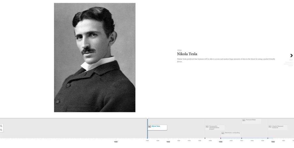
Big Data Evolution with TimeMapper
Today we will review an easy way to display some data according to a timeline in three steps:
Although sometimes it’s possible to use another type of visualization, if you don’t have too much time, TimeMapper may be a good option.
- In this example, you only have to prepare a spreadsheet on google drive with the following columns:
https://docs.google.com/spreadsheets/d/1gQSS4qHq9tqbadibaxyxg-VlI8H7wOcPuQhPYlnkzu8/edit#gid=0
I collected the information from Dezyre web: web: http://www.sabatebarcelona.com/productos/decoracion-de-interiores/wall-papers-vinilo-3m-hp-latex-decoracion-interiores/
2. Once you publish your file from drive:

3. Then you simply have to enter the link in the configuration page of TimeMapper and decide a title for your timeline:

And at the end, just publish it and here it is your timeline:
Quick, easy and a different option to explain a story.
This is not an amazing visualization
This does not pretend to be an deep and extensive visualization experiment. I just wanted to share with you a simple exercise of data visualization using Tableau.
I have to admit that my first contact with the tool was few months ago, and I also have to say that it has improved a lot this past year, adding some useful functionalities. (I have to admit that the video tutorials might have had something to do with this, but to tell the truth I’m falling in love again)
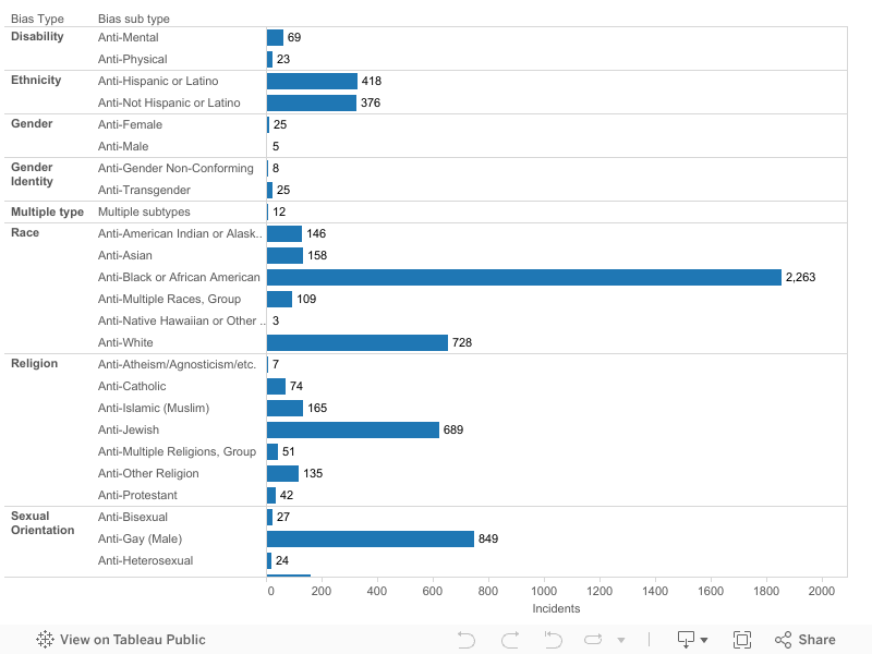
The visualization shows a representation of the offenses committed during 2013 by the bias motivation from the crime datase of the FBI.
The offenses (committed in 2013 in the USA) were grouped depending on the type of the offense: by race, religion, sexual orientation, even gender. Every type was subdivided in subtypes: by talking about religion we have more information about if the incident was done against catholics, jews, islamics, etc.
My first representation was just about the number of the incidents depending on the incident type:
Then I added the subtype variable to the color filter to add more deep information to every listed type:
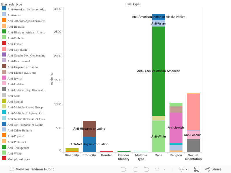
Not many conclusions about this , I simply want to say that is rather sad that the incidents related to race are still the most frequent, and that the number of offenses against the afro-american population triples the number of offenses against white people. The number of incidents related to race are followed by offenses linked to sexual orientation. Most of them against the gay community.
My boss is a troll
Well, not really a troll. A Troll by definition is a person that publishes wind-up messages in an online community with the main intention of annoying or provoking an emotional answer in the users or readers.
- Provocative message? Guilty.
- Trying to provoke an emotional answer? Guilty.
- Message Irrelevant? Not at all.

The conflict began on 4th of August with this first tweet in response to an infographic published on the El País twitter account:

in which apparently the most expensive signings from 1998 to 2015, between the English league and the Spanish league clubs were compared.
I say apparently, because it seems the information was wrong: Someone called Bale hadn’t been included. I have to admit I don´t know anything even about his existence and much less about football signings.
The second tweet (persistent) was this:

showing some Tableau created graphics using some data taken from The Guardian: Totally different results.
And the last tweet:

Giving as a reference and article with the same (and correct) numbers.
Wrong processing? Some kind of error? May be something deliberate?
After sitting in front the great Julio Pomar for months I know that’s not the best way to deal with a troll. By ignoring him, I mean, specially when the troll is telling the truth and we have published some wrong data.
The best way to react would had been to admit the error, say sorry and rectify the data.
Talking with my boss about that two weeks ago, I knew the reason for this unpleasant comment (I have to say that’s not his usual way of doing things. He is actually nice, respectful and always ready to help anybody):
“I think that journalists have access to a lot of information, information that most of us don’t normally have access to, so they have a commitment with the society to be honest and unbiased. Those things made me indignant.”
So I decided to write this post, and I might mention the author (@rodrigo0silva) in a tweet linking to this article. I probably won’t get an answer.
The Book of Trees: Visualizing Branches of Knowledge
The Book of Trees covers over 800 years of human culture through the lens of the tree chart, from its roots in religious medieval exegesis to its contemporary, secular digital themes. With more than 200 images the book offers a visual evolution along history of this universal metaphor, showing us the recent emergence of new visual models.

This book, written by Manuel Lima (Visual Complexity) makes visualization a prism through which we can observe the evolution of culture.

Manuel is a leading voice on information visualization and has spoken in numerous conferences, schools and festivals around the world, including TED, Lift, OFFF, Eyeo, Ars Electronica, IxDA Interaction, Harvard, MIT, Royal College of Art, NYU Tisch School of the Arts, ENSAD Paris, University of Amsterdam, MediaLab Prado Madrid. He has also been featured in various magazines and newspapers, such as Wired, New York Times, Science, BusinessWeek, Creative Review, Fast Company, Forbes, Eye, Grafik, SEED, Étapes, and El País.
The Data Visualization Catalogue
If you ever asked yourself which is the best type of visualization for your data, The Data Visualization Catalogue could provide a guide to help you decide.
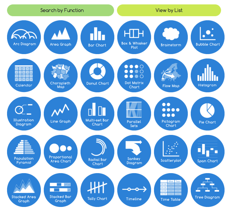
Severino Ribecca has begun the process of categorizing data visualizations based on what relationships and properties of data they show. With more than 50 types of visualizations, this catalog aims to be a comprehensive list of visualizations, depending on what you want to show.
The site has the potential to be a good reference for those looking to find the most efficient way to display data, or a new point of view to find different patterns or insights to understand what we need to communicate the meaning and the purpose of our data.
A.Track.Tion: How we Did it?
What music do people listen to? How does their taste change with time? Where do new music styles come from? In this post we go through the methodology and technique used to create A.Track.Tion, a data visualization aimed at shedding light on these deep and interesting questions.

Data gathering and processing
Our objective was to measure and visualize music popularity. As a proxy, we settled on the industry’s definition: popular music sells. As our core dataset, we started with the Whitburn Project list: a collective effort to gather historical weekly music sales rankings published by the Billboard company (the project is now maintained at the Bullfrogs Pond). The list goes back up to 1890, even though the Billboard’s Top 100 data officially starts after 1954. The dataset required a little cleaning, as some songs have inconsistent date formats, and others are missing their weekly position in the chart. The subset we used (only songs after 1954, and dropping a couple thousand incomplete records) contains 33560 songs.
The Whitburn Project has received attention before, with visualizations of song duration, one hit wonders, or more recently the obscurity of hit songs.
For our purposes, however, the data was incomplete in two ways:
1) First, we do not have sales data, at least directly: the Billboard company only publishes weekly rankings, which are ordered by some formula that depends on total sales. The formula has become more complex in the last two decades, as online presence is also taken into account. We need to invert this unknown formula (ok, not fully unknown, but it changes not only through the years but even week to week so it might as well be unknown to us). For this reverse-engineering , we used some publicly available sales data for a few weeks and years (like this, this, or this). The data is scarce (the company that measures it, Nielsen Soundscan, sells the subscription service to record companies and alike, and probably is expensive). However, we are optimists and we shall try to estimate from this the percentage of sales that a given ranking position entails. First, many many rankings based on economic figures follow a power law (also known as a Zipf’s law). Indeed our sales data shows a power law, but the two problems of power laws are also visible: One, for small numbers the power law tapers off (because real things do not diverge at zero), and two, for large rankings the tail is strange, specially if you have few data points like we do. However, we can optimistically say that the curves follow more or less the same slope, which means they follow the same power law! We estimate this slope to 0.75, that is, the sales follow a law such that sales = C * rank^0.75, where C is a normalization factor.

By choosing C so that all sales add up to 100, we have a convenient estimator of the percentage of sales associated with a given position in the weekly ranking. We just need to remember that for top 5 or so positions we overestimate the sales, and that the whole thing is just an estimate anyway — fitting more elaborate functions is not fully justified without bigger data. See below for a sanity check on our estimator.
2) Our second problem is that the original database contains only partial information about the genre of each song: only a few broad genres are listed, and only for a small percentage of the songs. To find this genre information, we searched and parsed thousands of Wikipedia articles, one for each song and artist in the list, and in this way collected data about the genre (or genres) that people have assigned to each song. This new dataset is actually richer than the original assigned genres, as many songs are now cross-genre, or they belong to niche sub-sub-genre of a broader music style (hello cowpunk). We found almost 800 musical genres, many associated to the songs in the database, and the rest because it was directly related to a genre already in the database (this, and rounding to zero, lead to some genres in the final plot appearing as having 0% popularity. We are working on fixing that). Because our parser was a little crude and naive, we had to curate and clean the list manually, separating actual genres from text the parser thought was genres (like the names of record companies). During this manual clean-up we also cleaned and re-assigned the relationships between genres. We think that it would not be so hard to perform an automated search and parse to complete our list.
Coupling our improved genre information with our estimate for percentage of sales, we are now able to estimate the percentage of sales for each musical genre and subgenre. Because many songs were linked to multiple genres, we decided to split the popularity equally among them.
The last piece of the puzzle is to connect our estimated percentages to actual money figures. For this, we will rely on the estimations of the global number of recorded music sales by the TsorT World Music Charts compilations. These estimates are very useful because they go way back to 1954, and they are close to the actual self-reported numbers from the industry: For 2007, TsorT estimates over 24 billion USD in total world sales, while the industry reported 19.4 billion USD. We normalized the TsorT data with this figure. TsorT only estimates up to 2007, for following years we used: 2008, 2009, 2010, 2011, 2012, and 2013. All our figures are inflation adjusted to 2013 US dollars.
Some results and sanity check
Our sales estimator allows us to compute the aggregated popularity for songs over several weeks (which assumes that total volume of sales is roughly constant over the period). This gives us an interesting opportunity to cross-check our sales estimator, and at the same time gossip and compare artists and songs! How can we pass this chance.
Why can we cross-check? Well, it turns out that Billboard itself has done the same calculation and published (for their 50th aniversary, and many times, actually) an all time ranking of songs. This is the one that betters compares to our time range (1955-2013). The Billboard list of top 20 songs:
- «The Twist» – Chubby Checker
- «Smooth» – Santana feat. Rob Thomas
- «Mack the Knife» – Bobby Darin
- «How Do I Live» – LeAnn Rimes
- «Party Rock Anthem» – LMFAO feat. Lauren Bennett & GoonRock
- «I Gotta Feeling» – The Black Eyed Peas
- «Macarena (Bayside Boys Mix)» – Los Del Rio
- «Physical» – Olivia Newton-John
- «You Light Up My Life» – Debby Boone
- «Hey Jude», The Beatles
- «We Belong Together» – Mariah Carey
- «Un-Break My Heart» – Toni Braxton
- «Yeah!» – Usher feat. Lil Jon & Ludacris
- «Bette Davis Eyes» – Kim Carnes
- «Endless Love» – Diana Ross & Lionel Richie
- «Tonight’s the Night (Gonna Be Alright)» – Rod Stewart
- «You Were Meant for Me / Foolish Games» – Jewel
- «(Everything I Do) I Do It for You» – Bryan Adams
- «I’ll Make Love to You» – Boyz II Men
- «The Theme from ‘A Summer Place'» – Percy Faith
And the list coming out of our estimator:
- «Smooth», Santana
- «I Gotta Feeling», The Black Eyed Pea
- «Macarena (Bayside Boys Mix)», Los Del Rio
- «We Belong Together», Mariah Carey
- «Un-Break My Heart», Toni Braxton
- «Yeah!», Usher
- «One Sweet Day», Mariah Carey
- «I’ll Make Love To You», Boyz II Men
- «Somebody That I Used To Know», Gotye
- «Candle In The Wind 1997», Elton John
- «Something About The Way You Look Tonight», Elton John
- «Party Rock Anthem», LMFAO
- «We Found Love», Rihanna
- «Low»,Flo Rida
- «Call Me Maybe», Carly Rae Jepsen
- «End Of The Road», Boyz II Men
- «I Will Always Love You», Whitney Houston
- «Boom Boom Pow», The Black Eyed Peas
- «Rolling In The Deep», Adele
- «The Boy Is Mine», Brandy & Monica
We observe that we have many of the songs in similar or close positions (mental note: we can do a visualisation of how the songs change positions between Billboard’s list and ours). Our biggest problem seems to be that we are miscalculating the popularity of some older songs («Hey Jude» comes in at position 79 in our list, what a disgrace to The Beatles), but we knew this would be a problem because Billboard has changed their methodology a few times in the past, and our data could be seriously skewed to newer songs (and in fact Billboard mentions explicitly that «certain eras are weighted differently»). This is probably why «Te Twist» is Billboard’s top song, and it only comes in at position 344 in our list…However, given our rough estimations, that we do not change our formula, and that Billboard applies a liberal dose of subjective-hand-adjusting to their data, we are quite satisfied with the level of agreement.
Billboard also has a list of top 100 artists that we can compare too. Their 20 first artists in the ranking are
1 THE BEATLES
2 MADONNA
3 ELTON JOHN
4 ELVIS PRESLEY
5 MARIAH CAREY
6 STEVIE WONDER
7 JANET JACKSON
8 MICHAEL JACKSON
9 WHITNEY HOUSTON
10 THE ROLLING STONES
11 PAUL MCCARTNEY/WINGS
12 BEE GEES
13 CHICAGO
14 USHER
15 RIHANNA
16 THE SUPREMES
17 DARYL HALL JOHN OATES
18 PRINCE
19 ROD STEWART
20 OLIVIA NEWTON-JOHN
while our list is
- Elvis Presley
- Mariah Carey
- Madonna
- The Beatles
- Usher
- Elton John
- Rihanna
- Whitney Houston
- Michael Jackson
- Stevie Wonder
- The Rolling Stones
- Katy Perry
- Janet Jackson
- Bee Gees
- Boyz II Men
- Nelly
- Prince
- The Black Eyed Peas
- Rod Stewart
- R. Kelly
We are very happy with the agreement.
Implementation
D3.js has been the bestest of friends. We love you Mike Bostock, and also the rest of lovely helpful people that helped us so much by posting examples online.
We created A.Track.Tion online, but we showed it on a large touch screen table at Sónar+D 2014, where it had a great reception by the festival audience as well as the music experts.

Limitations
Our dataset and our processing imposes a few limitations that we are aware of (and probably some we haven’t realised yet).
One large gap was already discussed, we still don’t have all possible musical genres listed in Wikipedia, but only those that we were able to crawl from our songs list. There are many more, and maybe some relationships (as older music styles start appearing) will change. For example, Jazz and Rock and Roll are said to derive from Blues, which in turn comes from American Folk Music.
Another large blind spot is that our database lists only songs that ranked in Billboard’s lists, which does not carry classical music and other styles. Those are indeed popular, but we do not have info to include it. Furthermore, the lists only include US sales, which further limit our findings to American musical taste (which is why Country music is so popular), and introduces a few strange oddities («world music», for example).
On the influence between genres, notice that we can only count how many genres have been influenced by a particular one, but this does not correlate (probably) to how many records have been produced on each genre, or how many musicians work on it.
Another criticism we received while at Sónar+D from music professionals was that we based our influence and genre information mostly on Wikipedia, instead of some other list curated by experts. While there is some truth to this (Wikipedia has been known to contain a few errors now and then), we found the curated hierarchies to be much more structured and similar to a tree, and most songs associated to a single genre. We think this is artificial, and that the complexity of the Wikipedia data reflects better the reality of music.
Another clear limitation is our sales estimator, which we produced from a rather small dataset (small in time, space, and number of records). Also, since the formula used by Billboard has changed many times in the past, we cannot expect it to hold for all our data. Perhaps we could find and produce a better estimate, but for our purposes our estimation is already good enough.
(EDIT) Note: We are aware of a small bug in the processing scripts that lost a few hundred records due to some text appearing in the original database where numbers were expected (in the position by weeks columns, if you need to know). We are working to fix this asap.
Acknowledgements
We thank the many anonymous contributors to the Whitburn project, and BSC for supporting this project.
